In my previous post I demonstrated using a variant of Hinton diagrams to visualize complex matrices at a glance. In my opinion, these diagrams are far superior to numpy array printouts for 90% of the times I need to inspect a matrix (and would probably be superior in all cases if augmented by a tooltip that displayed value in decimal notation when hovering over a particular element). However, for the specific case of visualizing SU(3) representations I think we can do better. The use of a matrix to represent a linear map imposes an ordering on the basis vectors, which is fine for SU(2) where there is a natural ordering on the basis vectors, but is pretty arbitrary in the (3, 0) Fourier transform example I used in the previous post (300, 210, 120, 030, 201, 111, 021, 102, 012, 003).

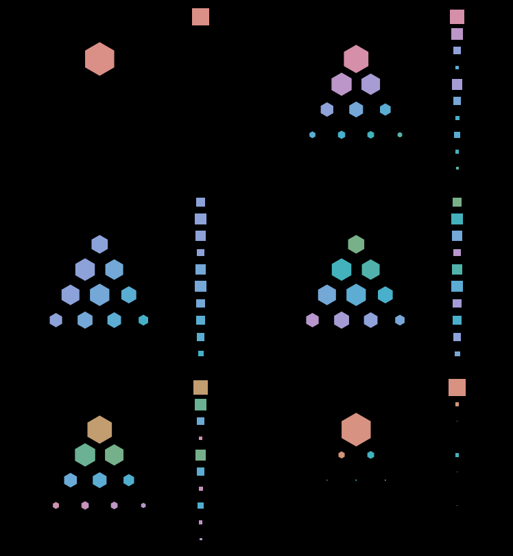
To overcome this representational issue, let’s start by considering how we represent a vector. Typically, we use a column vector, which exhibits this ordering of the basis elements. For SU(3), though, I suggest we take our cue from weight diagrams, which lay out the basis elements for an SU(3) representation in two dimensions.

In the $(p,q)$ irreps with both $p$ and $q$ nonzero, this representation has difficulties since some of the weights have multiple weight vectors associated with them, but for the $(p,0)$ irreps these triangular grids are a wonderful way to lay out the basis elements. One can then represent a vector in a $(p,0)$ irrep by adapting the complex Hinton diagram to the triangular grid instead of the rectangular grid. I made a GIF using this representation to depict the orbit of the highest-weight vector 300 under a continuous family of SU(3) representatives generated by a Hamiltonian that defines a closed orbit in SU(3). This representation lets you see some things more easily, like when all the phases line up parallel to one of the triangle’s edges, as opposed to the representation when we lay everything out along a line, which I’ve included on the right for comparison.

The next step is to expand this vector representation into a representation for linear maps, which I’ll do next time.