I’m just back from Boston, where I presented some recent work¹ at the American Physical Society’s March Meeting. I’m still finishing the paper, so in the meantime for those interested I’m going to expand on some of the main points in the talk here on my blog.

Unattainable bounds

I warned in my talk that treating the problem of estimating a function of multiple parameters as a single-parameter estimation problem can lead you astray. You’ll generally calculate unattainable bounds and introduce unnecessary errors in your estimates. The unattainable bounds are discussed in a specific case in the paper² that inspired this work, which I collaborated on with with Zachary Eldredge, Michael Foss-Feig, Steve Rolston, and Alexey Gorshkov at the University of Maryland. Section III.B. of that paper goes into some detail about why naïvely calculated single-parameter bounds are generally unattainable for the sensor networks we considered. Here I present another illustration of the problem, because it never hurts to see something explained multiple ways!

A classical problem is simplest to get the point across. Imagine a two-dimensional family of Gaussian distributions parametrized by their mean and with constant covariance

$$\begin{aligned} P(\mathbf{x})&=\exp\left[-(\mathbf{x}-\mathbf{\mu})^\mathsf{T}\mathrm{\Sigma}^{-1}(\mathbf{x}-\mathbf{\mu})\right] \,/\,\sqrt{2\pi\,\mathrm{det}\mathrm{\Sigma}} \\ \mathbf{\mu}&=\begin{bmatrix}\theta^1 \\ \theta^2\end{bmatrix} \\ \mathrm{\Sigma}&=\begin{bmatrix}1^2 & 0 \\ 0 & 2^2\end{bmatrix}\,. \end{aligned}$$

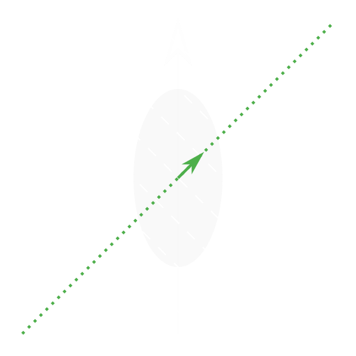
Given the ability to sample from a distribution from this family, how precisely can we estimate the sum $f(\theta^1,\theta^2)=\theta^1+\theta^2$? The picture below illustrates this problem.

If we treat this like a single-parameter problem, we’ll calculate the Fisher information for the sum using the partial derivative $(\partial_1+\partial_2)/2$ (since adding a half unit each of $\theta^1$ and $\theta^2$ is the most direct way to increase $f$ by one unit):

$$\int dx\int dy\frac{\left[(\partial_1+\partial_2)P(\mathbf{x})/2\right]^2} {P(\mathbf{x})}=\frac{1}{4}\left(\frac{1}{1}+\frac{1}{4}\right)=\frac{5}{16}$$

This suggests that fluctuations in $f$ ought to be $\sqrt{16/5}\approx\frac{441}{250}<2$. This agrees with the picture, where the shaded covariance ellipse doesn’t quite advance to the $f=2$ level surface along the greed dotted line depicting movement along $(\partial_1+\partial_2)/2$.

We know something about how our estimates ought to be constructed here, though. We should sample $\mathbf{x}=(x,y)$ many times and take the sum of the average of $x$ and the average of $y$. This distribution of estimates we will get with this procedure is the original distribution marginalized over lines of constant $\theta^1+\theta^2$, just with variance inversely proportional to the number of samples drawn. Calculate this marginal covariance by reparametrizing the distribution with $\mathrm{\Upsilon}_\pm=x\pm y$

$$\frac{1}{2}\int d\mathrm{\Upsilon}_+\int d\mathrm{\Upsilon}_-\,(\mathrm{\Upsilon}_+-\langle\mathrm{\Upsilon}_+\rangle)^2 P\left(\frac{\mathrm{\Upsilon}_++\mathrm{\Upsilon}_-}{2}, \frac{\mathrm{\Upsilon}_+-\mathrm{\Upsilon}_-}{2}\right)=5$$

This tells us that fluctuations in $f$ are actually $\sqrt{5}\approx\frac{9}{4}>2$, showing the calculation from the single-parameter approach is in error.

As I mentioned in my talk, this is because the single-parameter problem assumes additional parameters are fixed to known values. As the picture makes clear, if we actually knew $\mathrm{\Upsilon}_-=0$, then the conditional distribution for our estimates of $f$ would have fluctuations smaller than 2, but since we have uncertainty about $\mathrm{\Upsilon}_-$, we need to consider the marginal distribution, which has fluctuations greater than 2 (depicted as the covariance ellipse extending beyond the $f=2$ level surface).

I’m planning a follow-up post on the form of the optimal measurement strategy for the example given in my talk, but I’m also open to addressing other specific questions people raise.

---

1. One from many: Scalar estimation in a multiparameter context, 2019 APS March Meeting, Boston, MA, March 7, 2019 (abstract: K28.00012, slides)↩︎

2. Optimal and secure measurement protocols for quantum sensor networks
   Zachary Eldredge, Michael Foss-Feig, JAG, S. L. Rolston, and Alexey V. Gorshkov
   Phys. Rev. A 97, 042337 (2018), DOI:10.1103/PhysRevA.97.042337, arXiv:1607.04646↩︎