Gambler's Ruin

Over the summer, I took the opportunity to start watching through the lectures on the Perimeter Institute website on Quantum Foundations. During one of the lectures on probability, the following scenario was put forth:

Original Problem

Suppose I offer you the opportunity to place a bet on a toss of my coin. Placing a bet involves splitting your money between heads and tails. After the toss, the money you bet on the side that came up is doubled and returned to you (I get to keep the money you bet on the side that did not come up). You also know that my coin is more likely to come up heads than tails. Specifically, the probability $p$ that heads will come up lies in the open interval $(\frac{1}{2},1)$. What strategy should you use to place your bet?

Naïve Approach

The naïve strategy is to try and maximize the amount of money you make on average. To simplify calculations, let us assume your initial money is $G_0=1$, and let us denote the fraction of money you bet on heads by $y$. The money you make on average after one toss can be calculated as shown below:

$$\mathrm{E}[G_1]=2yp+2(1-y)(1-p)=2\big((2p-1)y+1-p\big)$$

Since $p>\frac{1}{2}$ means $2p-1$ is positive, this is maximized when $y=1$—i.e. when you bet all your money on heads. Using this strategy, on average you will make $\mathrm{E}[G_1]=2p>0$. Since you make money with this strategy on average, you will make even more money on average if you continue to place bets. After placing $N$ bets, the average money you will have is $\mathrm{E}[G_N]=(2p)^N$. This seems good, until you consider that with this strategy you will lose all of your money if only a single tails comes up. How likely is this to happen? The probability of not getting all heads for $N$ tosses is $1-p^N$, which very quickly approaches $1$ as you begin placing more bets. If you place bets ad infinitum, as this strategy tells you to do, you will certainly lose all of your money (hence the name, Gambler’s ruin).

Modified Approach

The question I wanted to answer was: is there a strategy that can take advantage of the bias of the coin without leading to ruin? To avoid the pitfall of the previous strategy, I wanted to find strategies that gave you a better chance of making money than losing money. Specifically, which values of $y$ give you a higher probability of making money than losing money as you place more and more bets?

My gut feeling was that there was a transition fraction $y_\text{trans}$ such that when betting many times if $\frac{1}{2}<y<y_\text{trans}$ you would most likely make money, whereas if $y_\text{trans}<y<1$ you would most likely lose money.

Numerical Investigation

Before embarking on an analytic pursuit of this transition, I decided to run a quick simulation of the scenario in python. When considering only a finite number of throws, the probability of making money can be calculated exactly. This is done by considering all sequences of coin tosses and summing the probabilities of those that result in you making money. To do that, we need to calculate the amount of money you have given a sequence of coin tosses. Suppose after a partial sequence $\mathbf{s}$ of tosses the amount of money you have is $G(\mathbf{s})$. How much money would you have after the next toss if it comes up heads? We double the fraction of money you bet on heads, so $G(\mathbf{s}\cdot H)=2yG(\mathbf{s})$. Similarly, if a tails had come up instead you would have $G(\mathbf{s}\cdot T)=2(1-y)G(\mathbf{s})$. These examples make it clear that each coin toss has the result of multiplying your previous amount of money by a number depending on the outcome. Since it doesn’t matter what order we multiply these numbers together in, we can see that it doesn’t matter what order the outcomes are arranged in. All that is important is how many times either heads or tails came up. From this, and the fact that we are defining our starting money $G_0=1$, we can calculate the money you have after $N$ tosses:

$$G_N(f)=2^Ny^f(1-y)^{N-f}$$

Here $f$ stands for the number of times heads came up (the favorable outcomes, if you will). For the purposes of our simulation, we also need to know the number of individual sequences where heads comes up $f$ times. This is given by the combinatorial expression $\binom{N}{f}$. The responsibility of our python program is now to calculate which values of $f$ result in $G_N>1$ for a given $y$, multiply the probability of getting a sequence with $f$ heads by the number of different sequences with $f$ heads, and sum all these probabilities together. We can calculate the probability of making money as:

$$P_\text{gain}=P(G_N>1)=\sum_{G_N(f)>1}\binom{N}{f}p^fp^{N-f}$$

My first program was a little clumsy in that it checked all values from $1$ to $N$ for $f$, when in reality once the minimum $f$ is found all higher values of $f$ will give $G_N(f)>1$ (getting more heads is not going to decrease your return). The following python code uses scipy to calculate the probabilities and matplotlib to display the results:

from matplotlib import pyplot as plt
from scipy.special import binom
p = 0.8           # Probability of getting heads
N = 1000          # Number of coin flips
y_samples = 1000
# Array of fractions of money to bet on heads between 1/2 and 1
y_vals = [1/2 + x/(2*y_samples) for x in range(1, y_samples)]
# Array of minimum numbers of heads required to make money
min_f_vals = []
# Find the minimum value of f for all betting fractions y
for y in y_vals:
    # Set f to the max value by default (guaranteed to be profitable)
    f_min = N
    for n in range(N + 1):
        if y**n*(1 - y)**(N - n) > 1/2**N:
            f_min = n
            break
    min_f_vals.append(f_min)
# For each y sum the probabilities of all f that result in gain times the
# number of sequences that give each desired f
gain_probabilities = [sum([p**f*(1 - p)**(N - f)*binom(N, f) for f in
                      range(f_min, N + 1)]) for f_min in min_f_vals]
fig = plt.figure()
ax = fig.add_subplot(111)
ax.plot(y_vals, gain_probabilities)
ax.plot([1/2, 1 - 1/y_samples], [1/2, 1/2], linestyle='--')
plt.xlabel(r'$y$')
plt.ylabel(r'$P_\mathrm{gain}$')
plt.show()

Running the code results in output like below:

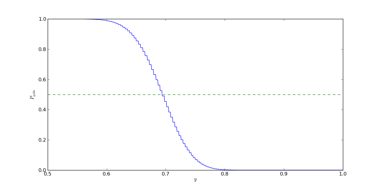
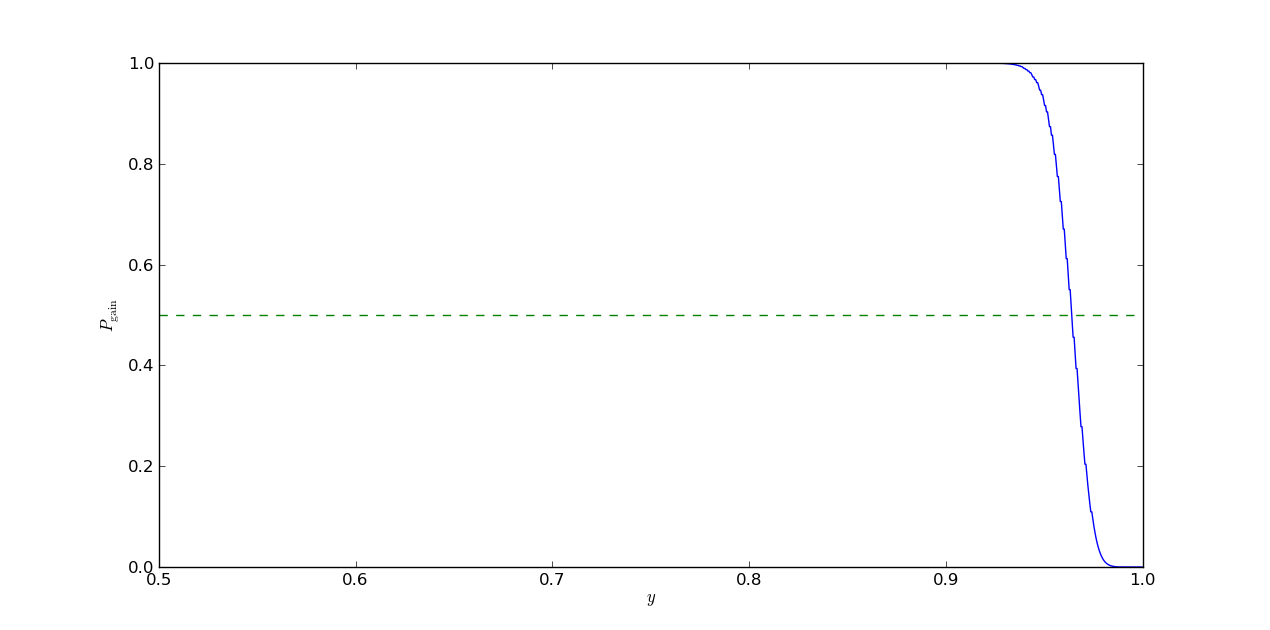
The value of $y$ for which $P_\text{gain}$ crosses the $\frac{1}{2}$ mark should approach the value of $y_\text{trans}$ as $N$ gets larger and larger. Playing around with various values for $N$, we see the crossing point becomes relatively constant as $N$ gets larger (the code I presented doesn’t do well for values of $N$ much higher than $1000$, likely because the exponentiation and binomial coefficients blow up). We also see the threshold is a function of $p$, as expected.

Analytic Solution

Computing the analytic solution involves taking the limit of infinite coin tosses to find which values of $y$ satisfy the following inequality:

$$\lim_{N\to\infty}P_\text{gain}>\frac{1}{2}$$

In this scenario we can employ the typical sequences theorem, which tells us that in this limit the probability that our sequence is in the typical set (where $\frac{f}{N}=p$) is equal to 1. Therefore, if sequences in the typical set have a gain greater than $1$ we will with certainty make money, and if they have a gain less than $1$ we will with certainty lose money. The value of $y$ for which the gain is equal to $1$ is the value at which we transition from making to losing money, and is what we are interested in calculating as $y_\text{trans}$:

$$G_N(Np)=2^Ny_\text{trans}^{Np}(1-y_\text{trans})^{N-Np}=1$$

If we take the logarithm of both sides and do a little rearranging, we find this expression equivalent to:

$$p=\frac{\ln2+\ln(1-y_\text{trans})}{\ln(1-y_\text{trans})- \ln y_\text{trans}}=F(y_\text{trans})$$

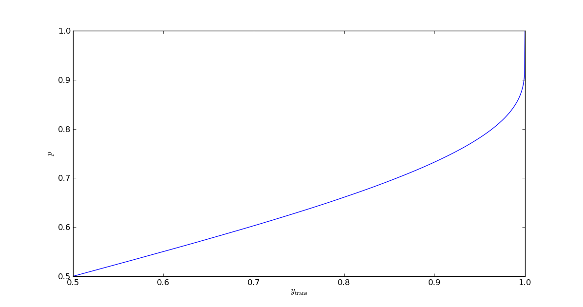
Unfortunately there is not a clean way to invert this function analytically. (If anyone knows how to represent $F^{-1}$ using well known special functions, I would be very interested to learn.) Fortunately for us, it is one-to-one on the open interval $(\frac{1}{2},1)$, so the inverse of the function exists and can be calculated numerically. With this inverse in hand, we can write:

$$y_\text{trans}=F^{-1}(p)$$

We have now solved our problem. Below are some plots showing the function $F^{-1}$ and overlays of the asymptotic $y_\text{trans}$ on top of the gain probabilities as a function of $y$ for various finite values of $N$.

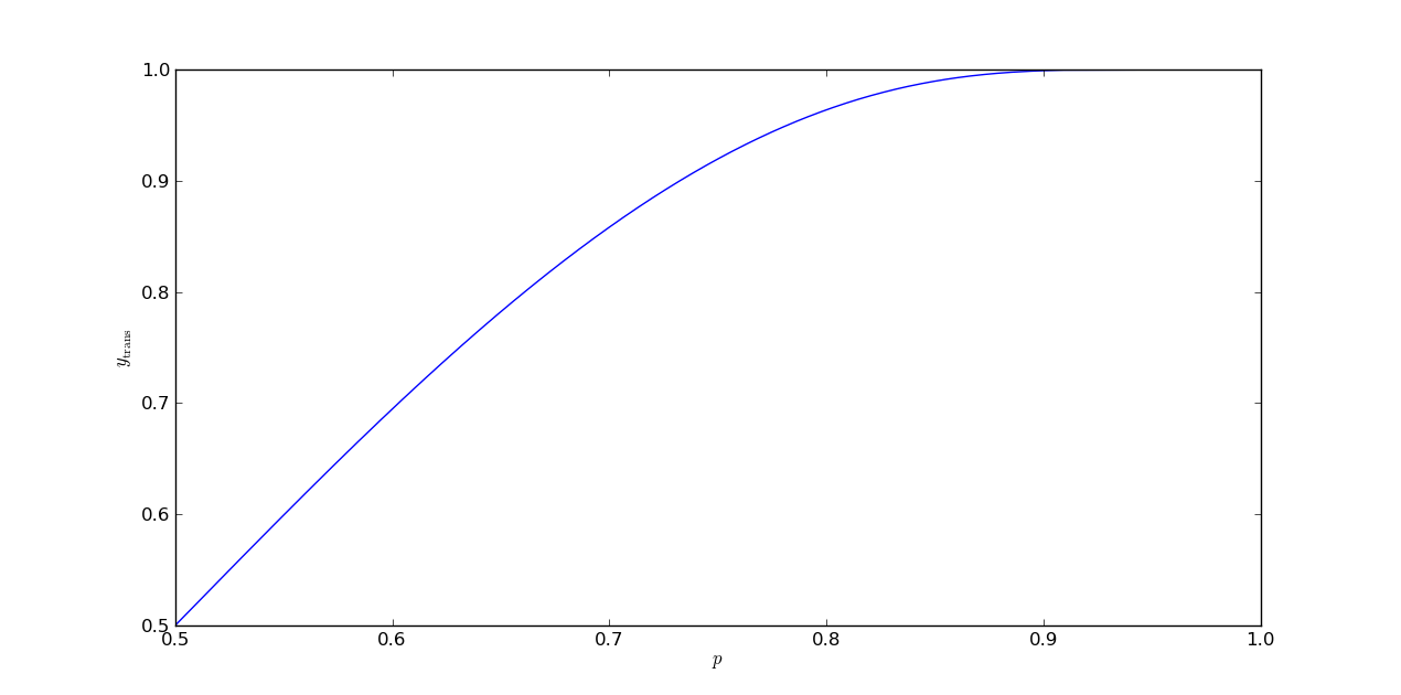
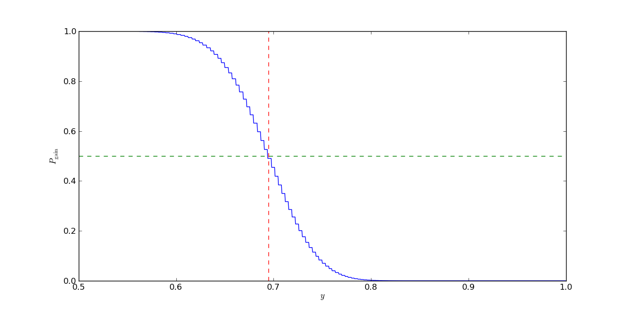
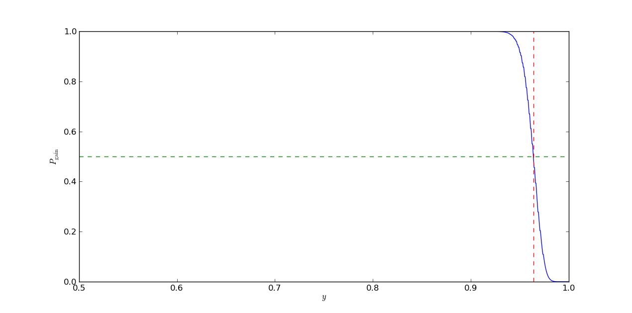
The values for $y_\text{trans}$ were calculated using a numerical zero finder from scipy.optimize:

y_trans = scipy.optimize.brentq(lambda y: (log(2) + log(1 - y))/(log(1 - y) -
    log(y)) - p, 1/2 + 1e-6, 1 - 1e-6)

As of publication, I don’t know of any other works that solve this specific problem, but I haven’t done a particularly exhaustive search either. If you know of one, please bring it to my attention and I will gladly reference it here.